Most manufacturing industries consume chemicals or plastics as raw materials or auxiliary materials in their production plants. To simplify this discussion, I will refer to chemicals and plastics together as chemicals.

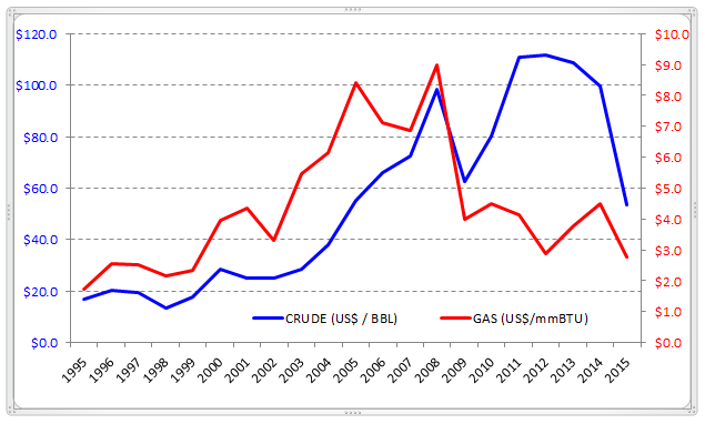
Since 2012, the peak year for oil prices, Crude Oil prices have fallen, and all chemicals users have enjoyed lower prices for Crude Oil derivatives. However, I believe this scenario will change in 2016 and 2017. In parallel fashion, Natural Gas prices have also fallen during same period, as shown in the graph below.  This is important to note as both feedstocks drive price movements for chemicals.

Background

Although several chemicals can be produced from Crude Oil or Natural Gas, most chemicals pricing follows Crude Oil prices. For example, Ethylene can be produced from Crude Oil or Natural Gas but follows Crude Oil prices, so producers of Ethylene using Natural Gas (at a lower price) enjoy a higher margin when Crude prices are high.

There are competing theories about the reasons for the Crude Oil price decline. Some conspiracy theorists believe the Organization of Petroleum Exporting Countries (OPEC) wants to financially restrict Iran and ISIS, which are both financed by oil exports. Others believe that OPEC wants to decrease the global oil inventory so the price will increase easily. My own view is that global oil prices declined in order to delay Shale Gas (mainly in the U.S.) investments and further production. Note: Shale Gas is Natural Gas in a different formation, which is cheaper than Crude.

Future

Any financial analyst of commodities or chemical specialist or, in fact, any person at large may try to predict the future. It is only after the fact, however, that we can realize who was right! So, I will give my view.

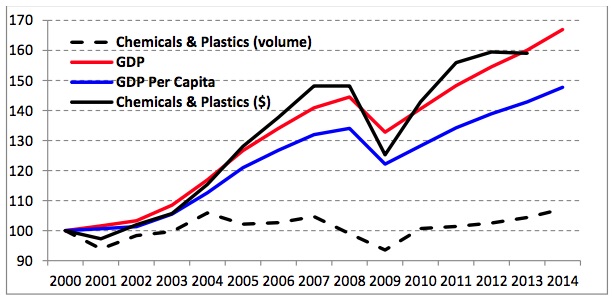
My first prediction concerns the chemicals industry in the U.S. This industry reported US$1,041 billion in revenue in 2014, and I believe it will reach US$1,400 billion in 2020, through a combination of price and volume increases.

My second prediction is related to Crude Oil. My view is that the Crude Oil price will reach an average of US$50/BBL in 2016 and US$60/BBL in 2017. As we all know, supply-demand balance defines the price, and in May, Bloomberg reported that OPEC ministers were “happy with the direction of the oil market” to “eradicate surplus production.” A second indication is the tremendous financial impact on the oil exporters. A recent Deloitte article provides a clear view of the impact on the budgets of oil exporters, showing they need a certain level of oil price in order to balance their internal budgets. Russia, for example, is heavily dependent on its oil revenues, with Oil and Gas accounting for 70 per cent of total export revenues. The country loses about $2 billion in revenue for every dollar fall in the oil price. The only oil exporter with high levels of monetary reserve to support this pricing environment is Saudi Arabia, and all others are struggling.

Assuming the oil prices as shown below, with Natural Gas around US$2.70/mmBTU, we may predict the following impact on Ethylene and Propylene.

The above predictions are based on statistical correlation analysis over the last 10 years.

Let us be very clear that the prices of Ethylene and Propylene are driven by the feedstock but also by the supply-demand balance of each one, as well as other derivatives. For example, Ethylene pricing depends on demand for middle-distillate products like gasoline, diesel, and heating oil. Additionally, propane pricing represents a ceiling price for Ethane. As result of all these drivers, Ethylene and Propylene prices have presented a delta (Propylene less Ethylene) between -$5 in 2000 to +$20 in 2011. Therefore, the prices may fluctuate much more than shown here.

There are several different chemicals, and the cost of each is driven by its feedstock as well as the supply-demand balance in that region. With that understanding, one approach would be to look at long-term historical data plus the delta range between the chemical and their feedstock and then relate these to the historical Crude Oil price. This would give an indication of how much your prices may increase.

For now, I propose you check these prices at the end of 2017 to see if I was right. If not, sorry; I just gave my view.

Taking Purchasing to the next level,

Paulo Moretti

In a recent article published at MyPurchasingCenter called Market Analysis: Chemicals and Plastics, I provided U.S. data for Chemicals & Plastics with past and future demand along with their growth rates.
In this follow-up article I will share global market data for Plastics with regional details for installed capacity, current and future demand, growth rates, imports, and exports. This aggregated market analysis was executed on 35 Plastics families totaling 340 million MT (750 billion lb.) of global products. A third article will cover Chemicals across the world.
It is critical for purchasing personnel to understand supply and demand of the products they buy, so they can advise their business partners of both the opportunities (lower cost) and the threats (supply disruption) in this space.

Background

The term Plastics is very broad and each reader will naturally relate to a different product. Here, I include as a Plastic any polymer (large molecule composed of many repeated subunits), thermoplastic or thermoset, elastomer, rubber, copolymer, or resin in any form (pellet, powder, liquid, etc.).
Plastics families include Polyethylene (LDPE, LLDPE, HDPE), PET, PP, PVC, Amino resins, Natural Rubber, PS, ABS, PC, PVA, Epoxy, Silicone, Acrylics, etc. Here I use the acronyms most widely known in the market.
In terms of regions, the data was aggregated as North America (USA, Canada, Mexico), Latin America (Central, South), Europe (Western, Eastern, Central, Baltic), Middle East and, Asia-Pacific (India, Southeast, Northeast, Oceania).
In terms of demand, the graph breaks this into “Current” and “Future” categories. Each market analysis has a different year as base line, with 2012, 2013, and 2014 being called Current. Future demand is considered five years ahead, correspondingly: 2017, 2018, and 2019. In a perfect world, we should have one single year as a base line, but different sources use different starting dates for their market data. In that regard, we need to see the data below in the perspective of magnitude and general direction, and not as a precise number.

Capacity & Operation Rate

The global capacity for all Plastics families is around 455 million MT (1 trillion lb.) where Asia-Pacific presents higher capacity than all other regions together as shown in Chart I.

Overall, Asia-Pacific represents the highest installed capacity in the world with 55% of 455 million MT, followed by Europe (17%), North America (14%), the Middle East (10%), and Latin America (4%).
In particular, the Asia-Pacific region leads in capacity of Natural Rubber (93% of global capacity), ABS (83%), PET (79%), SAN (77%), and Polybutylene Terephthalate (71%). North America leads in Sulfone Polymers (64%) and Polyvinyl Butyral (42%), and Europe in Polyisoprene (55%), Butyl Elastomers (40%), and LDPE (31%). Latin America and the Middle East do not lead installed capacity in any Plastics family.
Chart II captures the operation rates for each region.
North America presents the highest operation rate at 82% for the products produced in the region, followed by Europe (76%), Asia-Pacific (75%), Latin America (71%), and the Middle East (67%).
The analysis of operation rate can be considered under two perspectives: Unit Cost and Product Availability.

North America‘s higher percentage represents lower unit fixed cost (in manufacturing and expenses), compared to the other regions on the same basis. Basically, this is because we divide all fixed costs and expenses by a higher volume of products. However, each Plastics family presents a different impact of fixed costs on the total cost, as well as the magnitude of fixed costs from different sizes of the plants. For example, with Polystyrene, the unit fixed cost can be 10% to 16% (highest to lowest capacity) and with LLDPE, 33% to 42%.

The second perspective is to see where there may be more products available to buy from, in terms of percentage of capacity (not quantity itself). Of course, the quantity of 18% (available capacity) in North America capacity (11 MM MT) is higher than 29% in Latin America (5 MM MT). It is very probable that the region with lowest operation rate may offer a lower price in order to increase their capacity utilization (for example, the Middle East and Asia-Pacific).

Imports
It is important to turn our attention to the trade between regions. In part, imports reflect how a region covers its internal demand and also opportunity for purchases from lower-cost regions.

Asia-Pacific represents 50% of all importation of Plastics in the world and represents 27% of their demand. Regions with high percentage of imports (like Latin America and the Middle East) reflect the lack of local installed capacity. The Plastics families with high volume trading are PP (18 MM MT), HDPE (16), LLDPE (11), PVC (9), Natural Rubber (8), and LDPE (8).

Exports
Exports reflect the competitiveness of regions across the world.

As we see in Chart IV, Asia-Pacific is the biggest exporter because of its huge installed capacity. On the other hand, the Middle East and North America are areas that represent the highest export percentage compared to their installed capacity, showing their competitiveness based on lower feedstock costs.

Alert from China
• China‘s rise in status to big-time exporter (all products/services) is well documented, jumping from US$232 billion in 2000 to US$2,342 billion in 2014, a 10-fold increase.
• Recent McKinsey data showed China’s internal debt reached US$28 trillion (282% of their GDP), mainly driven by the housing market.
• During August/September 2015, China devalued the Yuan currency, and according to ValueWalk analysts, China may devalue up to 20% by 2016. Currency devaluation makes products cheaper.
• Asia-Pacific, mainly driven by China, has the biggest installed capacity (250MM MT) for plastics, and the region is operating at 75% of capacity. It has exported 43 MM MT, with still 63 MM MT to be produced.
• One conclusion from this information is that we may see more Plastics coming from China to help pay its internal debt.

Plastics Demand
All 35 Plastics families in my analysis present a Current demand (see Background note above) of 340 MM MT, which is expected to grow globally at a rate of 4.1% per year reaching 417 MM MT in the Future.
In Chart V, we see that the Asia-Pacific presents the highest global demand, both Current and Future, followed by Europe, North America, the Middle East, and Latin America.

The following nine Plastics families represent 80% of total Current demand of Plastics in the world: PET (60 MM MT), PP (58), HDPE (38), PVC (38), LDPE (20), Amino Resins (17), Natural Rubber, (11) and PS (10).

Growth Rate
In Chart VI, we see the Compound Average Growth Rate (CAGR) for the internal demand in each region. From a growth perspective, the Middle East has the highest rate at 10 MM MT, whereas Latin America has the third biggest rate at only 3.7 MM MT. Developed regions like Europe (lowest growth rate) represents 6 MM MT, and North America shows 6.7 MM MT. Again, Asia-Pacific has the highest impact on Future demand with 50 MM MT of Plastics.

In terms of Plastics families, the biggest growth rates are with Biodegradable Polymers (12.7%), Silicone (7%), Natural Rubber (5.6%), Polyvinyl Butyral (5.3%), and Polyamides (5%). Even with high growth, these Plastics have capacity available to attend the demand.

Conclusion
Although it is considered mature, the Plastics industry is still showing growth rates higher than GDP. This will be driven by consumer purchasing power improvement as well as convenience of plastics over other materials in our lives.
From the business perspective, it is imperative to understand the supply-demand of each Plastics family and the competitive position in each region in order to define long-term business strategy.
From the purchasing perspective, we need to educate ourselves about each Plastics family we buy at a granular level so we can select the suppliers that best fit our long-term needs, as well as identifying opportunity for lower-cost materials.

Taking Purchasing to the next level,

Paulo Moretti