Chemicals – Global Market Outlook
Chemicals – Global Market Outlook
This is the third of a series of articles related to global Chemicals & Plastics, links to the previous of which can be found here:
- Market Analysis: Chemicals and Plastics, U.S. data for Chemicals & Plastics with past and future demand along with their growth rates.
- Plastics – Global Market Outlook, Installed capacity, current and future demand, growth rates, imports, and exports.
Parallel to the second article, this global market outlook focuses on Chemicals, aggregating 116 Chemical families totaling demand of 3.0 billion MT (6.7 trillion lb.) of global products.
Background
There are thousands of chemical products on the market. However, the data from this market analysis are restricted to chemicals most consumed in the industry (in solid, liquid, or gas form) that are considered commodity chemicals.
In terms of regions, the data was aggregated as North America (USA, Canada, and Mexico), Latin America (Central, South), Europe (Western, Eastern, Central, and Baltic), Middle East, and Asia-Pacific (India, Southeast, Northeast, and Oceania).
An analysis of demand can be broken into “Current” and “Future” categories. Each market analysis has a different year as its base line, with 2012, 2013, and 2014 being called Current. Future demand is considered five years ahead, correspondingly: 2017, 2018, and 2019. In a perfect world, we should have one single year as a base line, but different sources use different starting dates for their market data. In that regard, we need to view the data below in the perspective of magnitude and general direction, and not as a precise number.
Capacity & Operation Rate
The global capacity for all Chemical families is around 3.1 billion MT where Asia-Pacific presents higher capacity than all other regions together as shown in Chart I.
Chart I

Overall, Asia-Pacific represents the highest installed capacity in the world with 48% of 3.1 billion MT, followed by Europe (20%), North America (19%), the Middle East (11%), and Latin America (5%).
The high capacity means, of course, a high market demand in the region, but also an alternative to import from that region.
Some of the chemicals present a higher capacity concentration in a specific region. Table A below shows which chemicals, in each region, have the highest concentration of global capacity (local capacity/global capacity). Having a higher capacity concentration may mean that the region has abundance and probably lower cost for that specific feedstock. It could also mean lower total unit fixed cost (manufacturing and expenses) because they produce higher volumes. Consumers of these products should consider sourcing from these regions.
| Table A – Percentage of Global Capacity | ||||
| North America | Latin America | Europe | Middle East | Asia-Pacific |
| Cellulose Acetate (54%) | Lithium (32%) | Oxo Chemicals (80%) | Bromine (48%) | Calcium Carbide (97%) |
| Propionic Acid (48%) | Ethanol (26%) | Ammonium Nitrate (55%) | Ethane (38%) | Acetylene (97%) |
| Ethanol (47%) | Potash (44%) | Chlorobenzenes (89%) | ||
| Sodium Chlorate (42%) | Propionic Acid (40%) | Sodium Sulfate (83%) | ||
| Ethane (38%) | Cellulose Ethers (39%) | Terephthalic Acid (81%) | ||
Chart II below captures the operation rates for each region. North America presents the highest Current operation rate at 82% for the products produced in the region, followed by Asia-Pacific (77%), Europe (75%), Latin America (74%), and the Middle East (71%).
Chart II

The analysis of operation rate can be considered from two perspectives: Unit Cost and Product Availability.
North America‘s higher percentage represents lower unit fixed cost (in manufacturing and expenses), compared to the other regions on the same basis. Basically, this is because we divide all fixed costs and expenses by a higher volume of produced products. However, each Chemical family presents a different impact of fixed costs on the total cost, as well as the magnitude of fixed costs from different sizes of the plants. For example, with Cumene, the unit fixed cost can be 5% to 7% (highest to lowest capacity) and with Sulfuric Acid, 61% to 75%.
The second perspective is to see which region may have more products available for purchase. Currently there is more product available from Asia-Pacific (469 million MT), Europe (181) and North America (131). It is interesting to note that product availability from Asia-Pacific is higher than total capacity from the Middle East or Latin America.
Imports
It is important to also pay attention to the trade between regions. In part, imports reflect how a region covers its internal demand and also provides opportunity for purchases from lower-cost regions.
Chart III

Asia-Pacific represents 51% of all importation of Chemicals in the world and represents only 11% of their demand. Regions with a high percentage of imports (like Latin America) reflect the lack of local installed capacity.
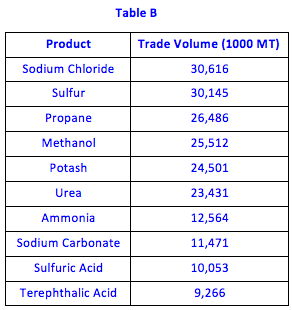
The Chemical families with high volume trading between the regions are shown in Table B and represent 63% of global trade volume of 116 Chemical families. The high volume tradable products are evidence that it is relatively easy to import and export products between regions and also that the prices between the regions are very similar. I believe that any company should buy from international sources in order to create competition with local suppliers and keep the prices in a lower level.
Exports
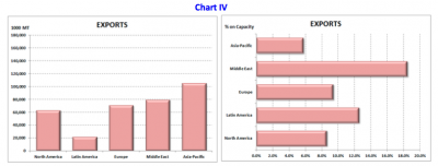
Exports reflect the competitiveness of regions across the world. As we see in Chart IV, Asia-Pacific is the biggest exporter because of its huge installed capacity. On the other hand, the Middle East represents the highest export percentage compared to their installed capacity, showing their competitiveness based on lower feedstock costs.
Chart IV
Chemical Demand
All 116 Chemical families in my analysis present a current demand (see Background note above) of 3.0 billion MT, which is expected to grow globally at a rate of 3.4% per year reaching 3.6 billion MT in the future.
Chart V

In Chart V, we see that the Asia-Pacific region presents the highest global demand, both Current and Future, followed by North America, Europe, the Middle East, and Latin America.
The Chemical families with highest demands in the world are shown in Table C. These chemicals represent 57% of all 166 Chemical families’ global demand.
Table C
| Product | Volume (1000 MT) | Product | Volume (1000 MT) | |
| Industrial Gases | 458,025 | Propane | 117,636 | |
| Sodium Chloride | 266,970 | Ethanol | 105,121 | |
| Sulfuric Acid | 243,473 | Propylene | 92,340 | |
| Ammonia | 143,057 | Urea | 83,365 | |
| Ethylene | 138,955 | Sulfur | 77,333 |
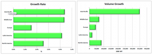
The Compound Average Growth Rate (CAGR), is the growth rate in percentage year over year in a specific region. It reflects the growth of all end-use applications of that specific chemical in a region, which of course, is driven by the overall growth of the region’s GDP. In Chart VI, we see the CAGR for the internal demand in each region, which shows Asia-Pacific, the Middle East, and Latin America with the highest growth rates. The same data from a volume perspective (see Chart VII) shows very clearly that Asia-Pacific is the region where chemical producers should have business, either by having local plants in the region or exporting chemicals from other regions.
Chart VI Chart VII
In terms of Chemical families, the biggest growth rates are described in Table D.
Table D
| Growth Rate | Product | Volume Growth (1000 MT) |
| 8.5% | Lactic Acid | 254 |
| 7.5% | Rare Earth | 49 |
| 7.5% | Activated Carbon | 507 |
| 7.5% | Methanol | 26,236 |
| 6.9% | Ethanolamines | 634 |
| 6.1% | Oxo Chemicals | 131 |
| 6.0% | Lithium | 51 |
| 5.7% | Cresols | 128 |
| 5.7% | Terephthalic Acid | 16,081 |
The growth rates at this level, much above GDP growth, reflect some new end-use applications or high growth rate from specific market segments. Every time we see a product with high demand where the supply is not following at the same rate, we can expect a price increase. This means that companies buying these chemicals may find difficulty getting the product if they do not have a contract in place.
Conclusion
Chemicals are used in all manufacturing industries as first or second tier materials, so it is important to understand market dynamics in the chemical world. From the chemical business perspective, it is imperative to understand the supply and demand of each Chemical family and the competitive position in each region in order to define long-term business strategy. From the purchasing perspective, managers need to educate themselves about each Chemical family they buy at a granular level, so they can select the suppliers that best fit long-term needs, as well as identifying opportunity for lower-cost materials.
Taking Purchasing to the next level,
Paulo Moretti